Research Problems in Pretraining

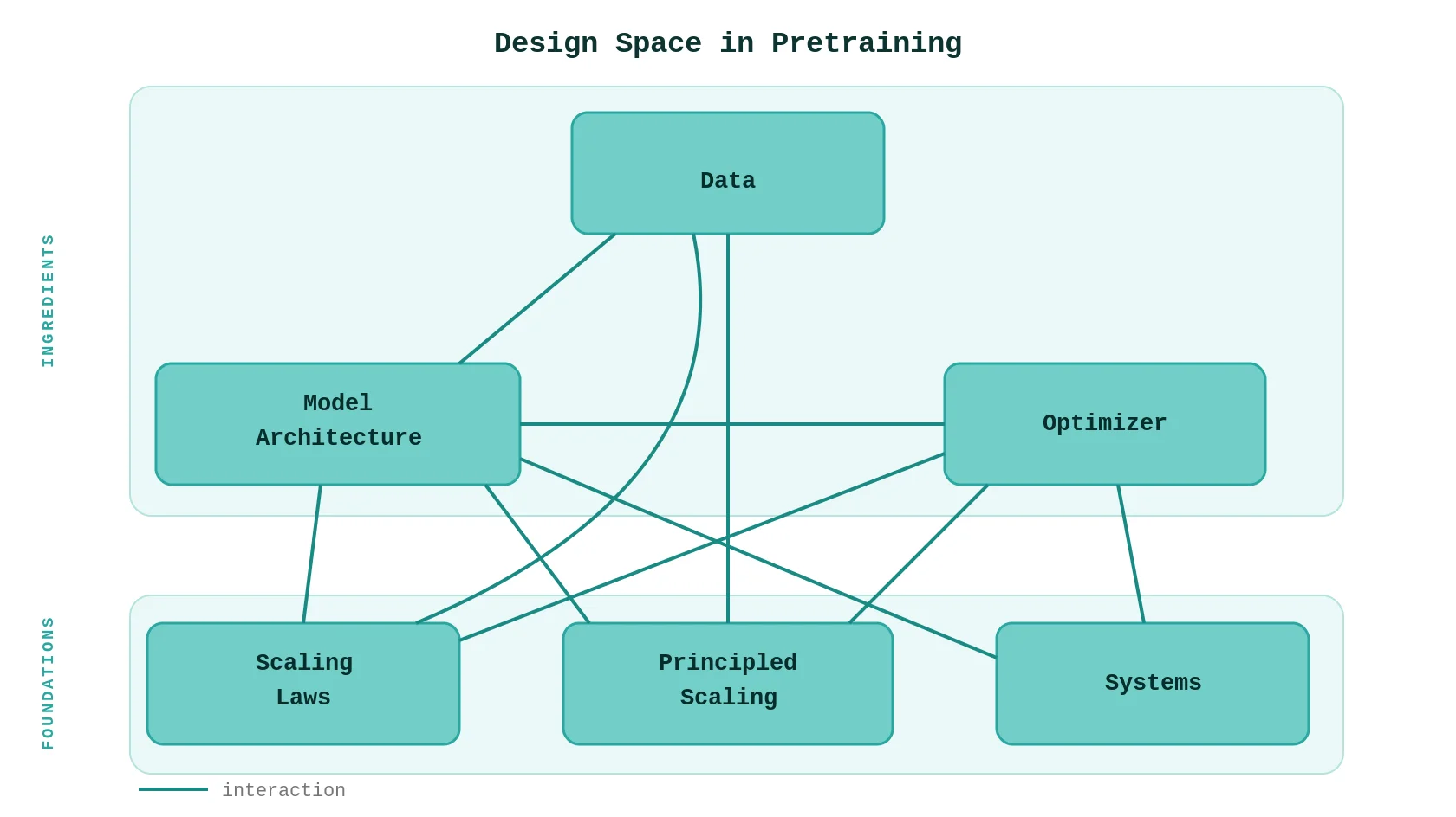
Most autoregressive language-model pretraining starts from the same objective: minimize next-token cross-entropy with a gradient-based optimizer. That objective does not specify the model, data mixture, optimizer configuration, or distributed execution plan. Choosing those inputs under a fixed compute and wall-clock budget is the research problem.

This post adapts my talk at the Stanford Math Department Student Learning Symposium.

The optimization problem

At its core, pretraining trains a model to predict the conditional distribution $P(x_{t+1} \mid x_1, \ldots, x_t)$ over a vocabulary, given a prefix of tokens. The loss is cross-entropy between the model’s predicted distribution and the ground truth. Training uses teacher forcing: at each step, the model conditions on the actual previous tokens from the training data, not its own predictions.

The objective predates modern language models. What changed is the scale of the models, token budgets, and distributed training runs used to optimize it.

The design space

I use six areas as a map of the design space:

1. Scaling laws — given a compute budget, how should you allocate between model size and data?
2. Model architecture — dense vs. Mixture-of-Experts, attention variants, KV sharing, hybrid local/global patterns.
3. Data selection and mixture — which data, in what proportions, in what order?
4. Optimizers — learning rate, batch size, scheduler, and the choice of optimizer itself.
5. Principled scaling / parameterization — how to transfer hyperparameters from small proxy models to the target scale.
6. Systems — parallelism strategies (tensor, pipeline, data, expert), MFU optimization, co-design constraints.

These are not six independent knobs. Architecture choices constrain feasible parallel layouts; data mixture can change optimization dynamics; and batch size affects both gradient noise and hardware utilization. In practice, teams hold most choices fixed while studying one treatment, then test the interactions most likely to change the decision. This article focuses on three cross-scale questions: predicting loss and architecture choices, transferring hyperparameters, and comparing optimizers and batch sizes.

Data quality deserves its own callout. In runs I have worked on, adding low-quality data has reduced how much target knowledge the model retained at a fixed token budget. I do not have a single controlled estimate that supports a general multiplier, so I treat this as a reason to measure interference rather than as a scaling law. Modern pipelines combine general deduplication with domain-specific filters, but many thresholds remain empirical choices. DoReMi formulates domain-mixture selection as minimax optimization, while RegMix uses regression over mixtures. Neither selects documents or defines quality for every downstream use.

The cost of being wrong

Consider a hypothetical sparse model with 100B active parameters trained on 100T tokens. The standard model-FLOPs approximation gives $6ND=6\times10^{25}$ FLOPs. An H100 SXM has approximately 1 PFLOP/s of dense BF16 Tensor Core peak throughput (NVIDIA), or about $3.6\times10^{18}$ peak FLOPs per hour. Assuming 20—35% MFU, the run requires roughly $4.8\times10^7$ to $8.4\times10^7$ H100-hours. If a planning model assumes $2.00—2.70 per H100-hour, that range becomes approximately $96M—226M.

Those numbers are scenario inputs, not universal estimates. MFU depends on architecture and layout; price depends on the contract and date. The $6ND$ estimate also excludes activation recomputation. Full-layer recomputation can add roughly one extra forward pass, about 33% relative to the usual forward-plus-backward approximation, while selective checkpointing adds less.

At that scale, architecture, data mixture, learning-rate schedule, and optimizer cannot all be grid-searched on the target run. Scaling ladders move those comparisons to smaller experiments, but only if their ordering extrapolates.

Scaling laws: the empirical backbone

Scaling laws model the empirical relationship between validation loss, model size, training data, and compute. Kaplan et al. (2020) documented power-law structure across these variables. Hoffmann et al. (2022) estimated a different compute-optimal allocation from a larger set of training runs, producing the “Chinchilla” result.

The Chinchilla form is:

$L(N, D) = E + \frac{A}{N^\alpha} + \frac{B}{D^\beta}$

where $N$ is model size, $D$ is the number of training tokens, $E$ is the fitted irreducible-loss term, and $\alpha$ and $\beta$ are fitted loss exponents. Under $C\propto ND$, this form gives $N_{\mathrm{opt}}\propto C^{\beta/(\alpha+\beta)}$ and $D_{\mathrm{opt}}\propto C^{\alpha/(\alpha+\beta)}$. Chinchilla’s parametric fit used $\alpha=0.34$ and $\beta=0.28$, implying allocation exponents of approximately 0.45 for parameters and 0.55 for tokens; its two other estimation methods produced values closer to 0.5 for both. Kaplan et al. had estimated $N_{\mathrm{opt}}\propto C^{0.73}$, allocating a larger share of additional compute to model parameters. These differences are empirical and depend on the fitted model family, data, and training setup.

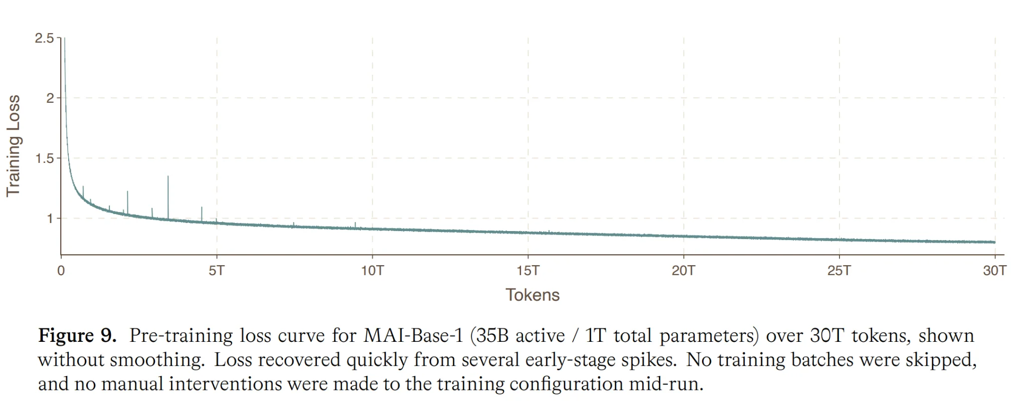From MAI-Thinking-1 technical report, Microsoft.

I have written separately about the math behind compute-optimal training in detail, including the derivation and its practical implications. Here I want to focus on how scaling laws are used in practice and where they break.

The MoE setting introduces additional dimensions: sparsity, granularity, expert count, and active parameters. Clark et al. (2022) extended scaling laws to routed models, and Krajewski et al. (2024) refined the functional forms further. Muennighoff et al. (2023) addressed the data-constrained regime, where tokens must be repeated.

The scaling ladder workflow

The practitioner’s workflow looks like this:

1. Train a “ladder” of small models at increasing compute budgets.
2. Fit the scaling law parameters to the observed losses.
3. Extrapolate to the target compute budget.
4. Use the extrapolation to set model size, data size, and other hyperparameters.

A ladder can be much cheaper than the target run, but the extrapolation distance must be reported. For example, a $300K ladder used to inform a $100M run represents roughly a 300-fold cost ratio; it does not by itself establish that the fitted curve remains accurate across a 300-fold compute increase. I track both the largest fitted compute and the target compute, hold out the largest ladder runs, and report prediction error on those held-out points before trusting the target extrapolation.

Two concrete techniques within this workflow:

Isoflop sweeps. Fix a compute budget. Train models of various sizes (adjusting token count to keep FLOPs constant). Plot loss vs. model size. The minimum gives you the loss-optimal model size for that compute level. Repeat at several compute budgets, and you trace out the compute-optimal frontier.

Treatment comparison. Fit parallel $L(C)$ curves for design variant A and design variant B. Extrapolate both to the target scale. The gap at the target is your estimated effect size. This lets you compare architectures, data mixtures, or optimizer configurations cheaply.

Where it gets hard

Signal-to-noise is the first problem. A treatment effect measured on one small model or one discrete benchmark may not preserve its sign at larger scale. I prefer continuous metrics where available, aggregate only tasks that measure the same capability, and repeat enough seeds to estimate whether the treatment gap is larger than run-to-run variance. Held-out ladder scales test whether the ranking survives extrapolation.

There is a deeper structural problem: the scaling laws for compute-optimality and for architecture optimization may use incompatible functional forms. Compute-optimal scaling relates loss to $(N, D)$. Architecture comparisons often need richer parameterizations. Joint optimization across both remains open.

The learning-rate schedule creates another extrapolation problem: a cooldown tied to a fixed token horizon makes intermediate checkpoints poor proxies for a run that decays at that point. Hägele et al. (2024) decouple cooldown from the stable training phase and test stochastic weight averaging (SWA) on stable-phase checkpoints. SWA improves those checkpoints and captures some effects of decay, but their experiments retain a gap to an explicit cooldown.

Finally, architecture comparisons must include attainable MFU. Two configurations can have similar predicted loss under the same model-FLOPs budget but require different GPU-hours because their best feasible layouts sustain different utilization. Under a fixed cluster allocation, compare predicted loss subject to the GPU-hour and memory constraints rather than ranking candidates by model FLOPs alone.

Principled scaling: from small to large

Scaling laws tell you what to expect at target scale. Principled parameterization tells you how to get there without re-tuning hyperparameters.

Under standard parameterization (SP), the scale of activations and updates changes with width. A learning rate tuned at one width therefore need not remain optimal at another. Which quantities remain stable depends on the parameterization, the layers being scaled, and the optimizer.

muP: Maximal Update Parameterization

Yang et al. (2022) introduced muP (Maximal Update Parameterization) for width scaling. It prescribes width-dependent initialization variances, learning rates, and output multipliers so that updates remain non-vanishing without diverging in the infinite-width limit.

Within the width-scaling setups evaluated in the paper, muP transfers tuned hyperparameters such as learning rate from smaller proxy models to wider targets. This does not imply automatic transfer across depth, architecture, data mixture, batch size, or optimizer changes; those dimensions require separate validation.

From Microsoft Research blog on muTransfer.

Everett et al. (2024) compared SP, muP, and intermediate parameterizations through width-scaling exponents for initialization and learning rate. Within the regimes they analyze, hyperparameter transfer is not unique to muP: other choices can transfer when the learning-rate scaling is adjusted appropriately. Under their alternative alignment assumptions, multiple parameterizations also admit feature-learning limits. The result makes muP one internally consistent transfer prescription rather than the only parameterization capable of transfer or feature learning.

Critical batch size

McCandlish et al. (2018) relate the critical batch size $B_{\text{crit}}$ to the gradient noise scale. Below it, increasing batch size can reduce the number of optimization steps with little loss of sample efficiency, assuming the system can process the larger batch in parallel. Above it, additional batch size yields diminishing reductions in step count.

Critical batch size links optimization theory to systems engineering: the best batch size depends on both gradient noise and hardware utilization.

Comparing optimizers across scale

Parameterization determines how optimizer hyperparameters should scale with width. Choosing the optimizer introduces a separate treatment whose data efficiency, parallel efficiency, memory use, and stability must be compared over the intended batch and model scales.

AdamW: the baseline

AdamW is a common baseline for language-model pretraining. It uses first- and second-moment estimates for per-parameter adaptive updates and decouples weight decay from the gradient update. Its broad use makes comparisons easier, but a scaling law fitted with AdamW does not automatically transfer to another optimizer.

Muon: spectral optimization

Muon (Jordan et al., 2024) takes a different approach, grounded in the theory of modular duality developed by Bernstein and Newhouse (2024). It applies a finite Newton—Schulz iteration to the momentum update, moving it toward the polar factor whose nonzero singular values are one. The iteration approximates that factor; it does not compute the exact nearest semi-orthogonal matrix. The weight matrices themselves are not constrained to be orthogonal.

The polar factor equalizes the nonzero singular values of each matrix update. This changes the geometry of the step rather than constraining the weight matrix itself. Later pretraining experiments report better data efficiency than AdamW at large batches, but the critical batch and throughput advantage depend on model scale, implementation, and distributed overhead. Muon is closely related to Shampoo, but uses the current accumulated momentum matrix rather than Shampoo’s running Kronecker-factor preconditioners.

Scion: the unifying view

Pethick et al. (2025) analyze a family of updates through Frank-Wolfe optimization over norm balls. In their formulation, a spectral-norm constraint yields a Muon-like polar update, while $\ell_\infty$ and $\ell_2$ constraints yield SignSGD-like and normalized-gradient updates.

This view supplies a common language for comparing update geometry. It does not establish that one norm is optimal for all Transformer layers or training regimes; that requires controlled scaling experiments.

Learning rate scheduling

Cosine decay is a common schedule, but it requires committing to a total training duration upfront. WSD (Warmup-Stable-Decay) instead uses a warmup phase, a stable phase at peak learning rate, and a short decay phase. Checkpoints from the stable phase can branch into separate decay runs, making continuation experiments and evaluation at multiple horizons cheaper.

Open theoretical questions

Power-law fits have held across many model and compute ranges, but their exponents and extrapolation error depend on the experimental setup. No existing theory explains all of those observations. Several partial accounts make different testable commitments:

The quantization hypothesis. Michaud et al. (2024) model learning as the acquisition of discrete quanta with different difficulty thresholds. A distribution over those thresholds can produce a power law. The open empirical question is whether independently measured skill acquisition follows the distribution required by the theory.

Learning curve theory. Hutter (2021) gives an information-theoretic account connecting power-law learning curves to properties of the data source. Testing it requires measuring whether changes in source structure predict changes in the fitted exponent.

Dynamical mean field theory. Bordelon, Atanasov, and Pehlevan (2024) derive scaling behavior in infinite-width limits. The practical test is whether its finite-width corrections predict the deviations observed in scaling ladders.

Simon et al. (2026) argue that power laws are one pillar of an emerging “learning mechanics,” a theoretical framework that would unify scaling, generalization, and optimization dynamics.

Beyond scaling laws, several questions sit at the frontier:

• Apparent emergence. A capability curve can look discontinuous because the evaluation metric is thresholded even when the underlying model behavior changes smoothly, as shown by Schaeffer et al. (2023). A useful experiment must separate metric-induced discontinuity from a change in the learned behavior.
• Hyperparameter transfer. For a chosen parameterization, which tuned quantities preserve their optimum across width, depth, batch size, data mixture, and optimizer changes? A held-out scale should falsify a proposed transfer rule before it is used on the target run.
• Architecture under a hardware budget. Which architecture minimizes predicted loss under a fixed cluster and training window, after memory and attainable MFU are included? For MoEs, this requires varying sparsity and expert geometry rather than treating active parameters as the only architectural coordinate.

What would change my decisions

For each target run, I want three predictions with held-out checks:

1. Loss and treatment ranking. Fit on the lower ladder rungs, then predict both loss and the ordering of competing treatments on a held-out larger rung. A ranking reversal invalidates the treatment extrapolation even if each loss curve looks smooth.
2. Hyperparameter transfer. Tune on proxy models, state which dimensions are supposed to transfer, and test the prescription at an intermediate scale. A shifted optimum defines the boundary of the parameterization claim.
3. Hardware-adjusted allocation. Predict memory, MFU, and wall-clock for each candidate layout, then compare those predictions with measured runs. A model favored by a model-FLOPs-only comparison but worse under the fixed GPU-hour budget should not be selected.

These checks do not solve pretraining jointly. They make the decomposition auditable: each small-scale result states what it predicts, the scale over which it is being extrapolated, and the observation that would prove it wrong.