Compute-Optimal Is Not Cluster-Optimal

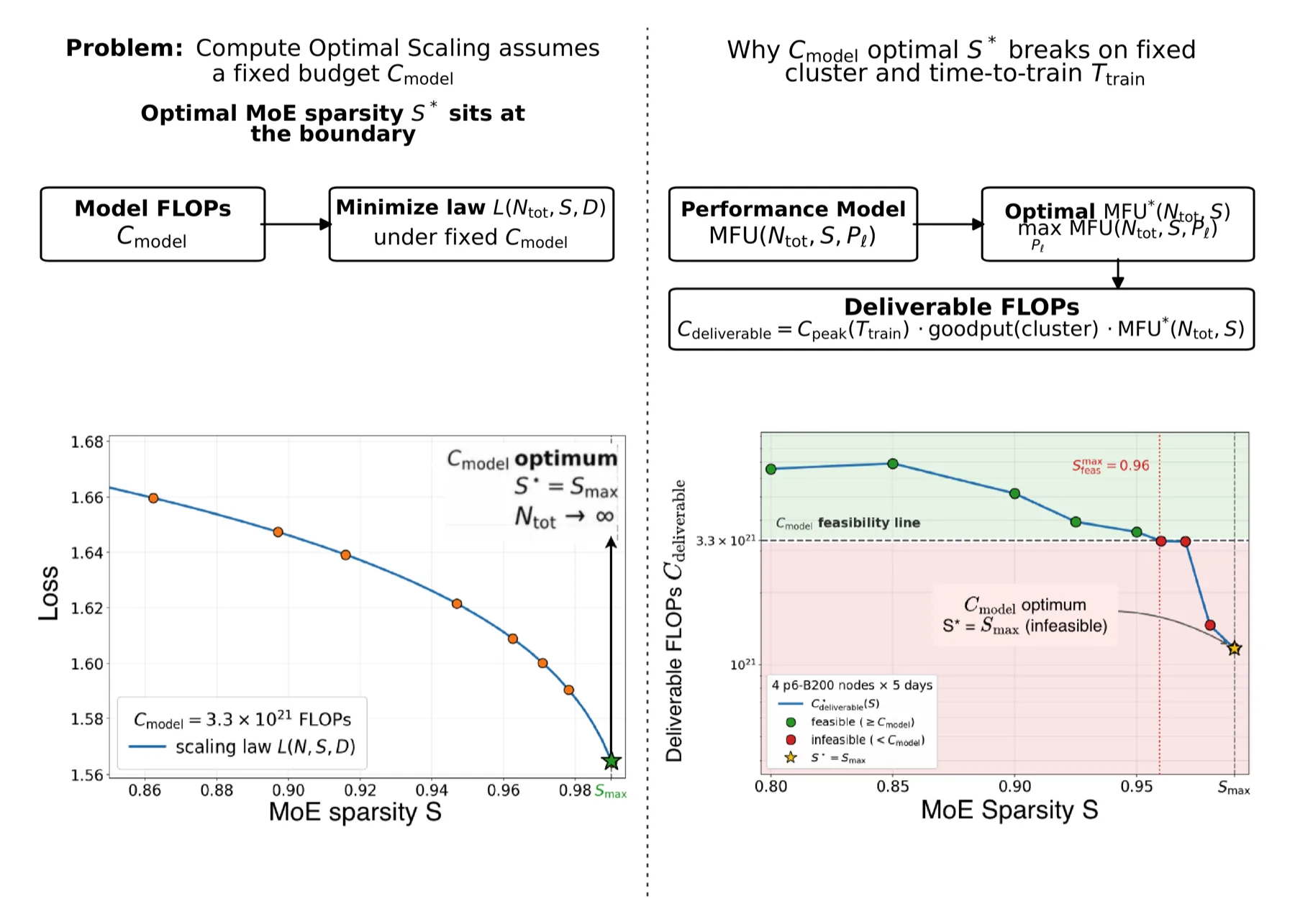
Pretraining design is usually split into two stages. A scaling law selects an architecture and token budget under a model-FLOPs constraint. Systems engineers then map that fixed architecture onto a cluster and optimize its parallel layout. This separation assumes that the cluster can deliver the prescribed model FLOPs independently of the architecture selected in the first stage.

That assumption fails when attainable model FLOPs utilization (MFU) varies across architectures. Two candidates with similar predicted loss at the same model-FLOPs budget can support different token budgets on a fixed cluster and training window because they sustain different MFU. Architecture selection must therefore account for the best feasible execution layout before fixing the training recipe.

Our paper, with Soumajyoti Sarkar and Yuxin Tang, introduces MOSAIC: a discrete co-design framework that jointly selects the architecture, training-token budget, and distributed layout for a specified cluster and wall-clock window.

From a model-FLOPs budget to a cluster constraint

Let $C_{\mathrm{peak}}$ be the raw compute ceiling determined by device peak throughput, device count, and training time. For architecture $Z$, layout $P_\ell$, and batch configuration $B$, MOSAIC defines

$$C_{\mathrm{deliverable}}(Z, P_\ell, B) = C_{\mathrm{peak}}\,\mathrm{MFU}(Z, P_\ell, B)\,\eta_{\mathrm{good}},$$

where $\eta_{\mathrm{good}}$ is the fraction of allocated time spent training. Unlike a conventional compute budget, $C_{\mathrm{deliverable}}$ depends on both the architecture and its layout. A training configuration is feasible only when its required model FLOPs do not exceed the maximum deliverable FLOPs over layouts that fit the cluster’s memory and parallelism constraints.

Sparse MoEs are where it breaks

A mixture-of-experts model replaces the dense FFN with a set of experts and a router, which decouples active parameters — the per-token FLOPs — from total parameters — the memory footprint. That introduces axes a Chinchilla-style law cannot see: sparsity, and the expert split factor $G$, which measures how finely the FFN width is partitioned into experts. The paper fits a joint law over total parameters, sparsity, tokens, and $G$ on roughly 150 from-scratch MoE pretraining runs, spanning 104M to 2.7B active parameters and total sizes up to 79B.

Under a fixed model-FLOPs budget, the fitted loss decreases monotonically with sparsity across the calibrated range. The optimum therefore lies at the upper boundary rather than at an interior sparsity.

The systems ordering runs in the opposite direction. At a world size of 512 GPUs, wall-clock time per delivered model FLOP rises monotonically with sparsity, reaching 1.70× that of the densest configuration. Along the expert-split axis, the corresponding maximum is 2.66×.

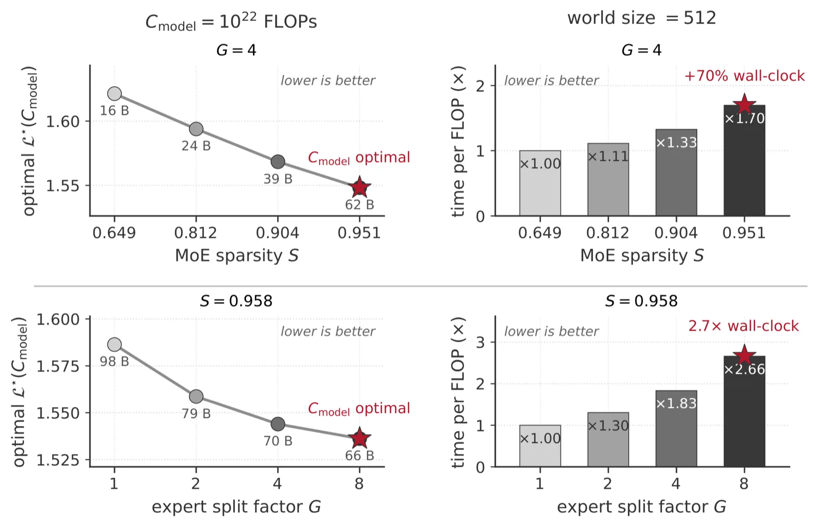The same design grid, scored two ways. At a fixed model-FLOPs budget (left), predicted loss favors sparser and finer-grained configurations. In wall-clock time per delivered model FLOP (right), those configurations are the slowest — 1.70× on the sparsity axis and 2.66× on the expert-split axis. From Figure 8 of the paper.

Joint architecture and layout selection

MOSAIC minimizes the scaling law’s predicted loss over discrete model geometries and token budgets, subject to the deliverable-FLOPs constraint. For each geometry, it searches feasible tensor, pipeline, data, context, and expert parallel degrees together with micro-batch size and activation checkpointing.

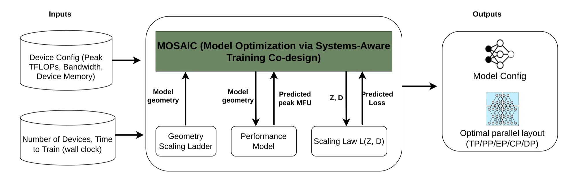The MOSAIC workflow. Cluster inputs enter on the left; a geometry ladder proposes realizable architectures; the performance model prices each in MFU and the scaling law prices each in loss. What comes out is a model configuration together with the layout to execute it. From Figure 2 of the paper.

The best layout for a fixed architecture is the feasible layout with the highest predicted MFU. Because loss decreases with token count, the token budget then saturates the resulting deliverable-FLOPs constraint up to the resolution of the search grid. These properties reduce the optimization to enumeration over the discrete architecture grid rather than a generic mixed-integer solve.

Consider a $3.3 \times 10^{21}$ model-FLOPs prescription on four AWS p6-B200 nodes for five days. The scaling law alone selects the upper sparsity boundary. On this hardware, configurations beyond approximately $S=0.96$ cannot deliver the computation required by that prescription within the training window.

Left: under a fixed model-FLOPs budget of 3.3 × 10²¹, predicted loss falls all the way to the edge of the calibrated range, so the optimum is the boundary. Right: the same prescription priced on four p6-B200 nodes for five days — past a sparsity of about 0.96, configurations deliver fewer FLOPs than the recipe requires. From Figure 1a of the paper.

Re-optimizing under the same envelope produces an interior feasible sparsity. Its predicted loss is 0.031 nats lower than the model-FLOPs boundary choice; no explicit maximum is imposed on a model dimension.

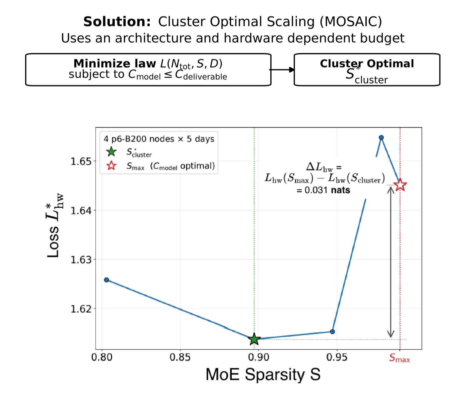Minimizing the same loss law subject to deliverable FLOPs produces an interior optimum (green star), 0.031 nats better than the model-FLOPs pick (red star) under an identical four-node, five-day envelope. From Figure 1b of the paper.

The inner search uses an operator-level performance model covering computation, collective communication, memory, and the 1F1B pipeline schedule. It is calibrated with target-hardware microbenchmarks and released as ScalePlan. On p6-B200 nodes, mean absolute percentage error for predicted MFU is 9.6%, 9.0%, and 13.2% for the 700M, 5.4B, and 18B active-parameter sweeps. Top-5 and top-10 overlap with measured rankings is 100% on every 5.4B and 18B sweep; the 700M sweep reaches 80% and 90%, respectively.

The candidate with the most FLOPs is not the best model

Under a 32-node, 20-day envelope, every candidate has the same raw ceiling of $9.95 \times 10^{23}$ FLOPs. The $G=8$ geometries have a median predicted MFU near 8%, while $G=2$ geometries reach 13—20%. In the Megatron-Core stack modeled here, finer expert partitioning incurs more dispatch and combine communication and therefore delivers fewer model FLOPs from the same hardware ceiling.

The candidate that realizes the most model FLOPs, $1.94 \times 10^{23}$, has higher predicted loss than the MOSAIC optimum. The optimum is a $G=4$, $E=96$, $K=2$ configuration with 14.5B active parameters and $S=0.956$. It reaches a predicted loss of 1.3898 using $1.23 \times 10^{23}$ model FLOPs, approximately 36% fewer than the highest-throughput candidate.

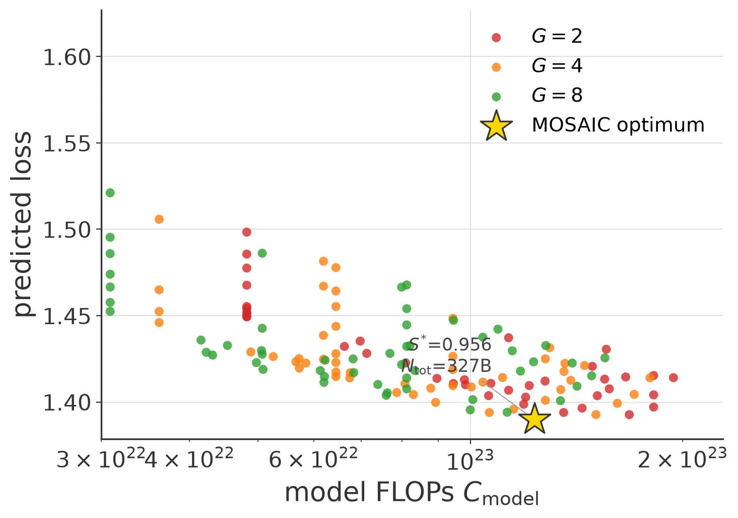Every feasible configuration under the 32-node, 20-day envelope, colored by expert split factor. All draw on the same raw ceiling, so a point sits further right only by sustaining a higher MFU. The gold star — the configuration MOSAIC returns — is conspicuously not the rightmost point. From Figure 10 of the paper.

Across the budget sweeps, optimal sparsity is not monotonic. It remains on a broad plateau from approximately 0.915 to 0.963. The optimal active-parameter count stays near 14—15B as the training window grows, then reaches 34B and 58B at the two largest cluster sizes. Near-ties at adjacent budgets leave the exact transition points unresolved.

The ordering survives contact with hardware

The paper also tests whether the predicted ordering transfers to hardware. Four configurations selected under an eight-node, ten-day envelope were launched as staged pretraining runs. They span up to 250B total parameters and continue beyond the selection envelope.

Measured MFU reproduces the predicted ordering across all four runs. For the two leading configurations, ID 2 leads over much of the lower model-FLOPs range, while the trajectories converge near $10^{22}$ model FLOPs and ID 1 slightly overtakes it within the width of the smoothed curves. On the peak-equivalent hardware-compute axis, $C_{\mathrm{model}}/\mathrm{MFU}$, ID 1 takes the lead earlier. Its normalized measured MFU is 0.84 versus 0.69 for ID 2, so it delivers approximately 1.2× as much model computation per unit of hardware compute.

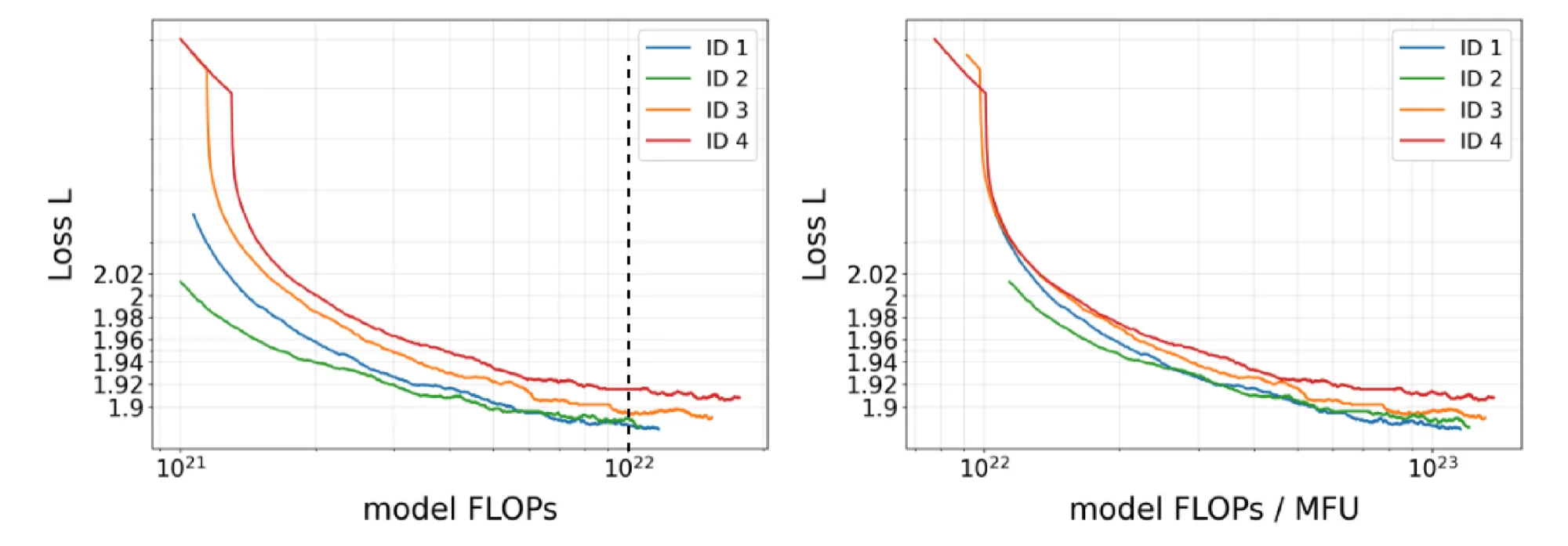Smoothed loss trajectories of the four staged runs. Left: against model FLOPs, ID 2 (green) leads over much of the range. Right: against peak-equivalent hardware compute, which divides out the MFU each run actually sustained, ID 1 (blue) takes over far earlier. The same four runs, ranked two ways. From Figure 12 of the paper.

What it does not settle

The specific geometries MOSAIC returns are conditional on the geometry ladder, the hardware platform, and the training recipe, and some reported optima sit beyond the regime the law was fit on. Uncertainty in the law’s non-identified coefficients is not propagated through the discrete search. The performance model mirrors a fairly basic Megatron-Core stack, so the absence of a clean trend in optimal $G$ may be that stack’s artifact rather than a property of MoEs — better kernels could change it. The evidence supports the hardware-aware ranking and the co-design principle more strongly than it supports any single geometry as a universal answer.

Implication for pretraining design

When attainable MFU depends on architecture, a model-FLOPs budget is not sufficient to rank candidates under a fixed cluster allocation. Architecture selection should jointly evaluate predicted loss, memory feasibility, and attainable MFU under each candidate’s best parallel layout. MOSAIC demonstrates this co-design procedure for sparse MoEs; the reported optima remain conditional on the evaluated model family, software stack, hardware, and training regime.